這篇文章將為大家詳細(xì)講解有關(guān)Pytorch搭建分類回歸神經(jīng)網(wǎng)絡(luò)并使用GPU進(jìn)行加速的案例分析，小編覺(jué)得挺實(shí)用的，因此分享給大家做個(gè)參考，希望大家閱讀完這篇文章后可以有所收獲。

創(chuàng)新互聯(lián)基于成都重慶香港及美國(guó)等地區(qū)分布式IDC機(jī)房數(shù)據(jù)中心構(gòu)建的電信大帶寬，聯(lián)通大帶寬，移動(dòng)大帶寬，多線BGP大帶寬租用,是為眾多客戶提供專業(yè)服務(wù)器托管報(bào)價(jià)，主機(jī)托管價(jià)格性價(jià)比高，為金融證券行業(yè)西云機(jī)房，ai人工智能服務(wù)器托管提供bgp線路100M獨(dú)享，G口帶寬及機(jī)柜租用的專業(yè)成都idc公司。

分類網(wǎng)絡(luò)

import torch
import torch.nn.functional as F
from torch.autograd import Variable
import matplotlib.pyplot as plt

# 構(gòu)造數(shù)據(jù)
n_data = torch.ones(100, 2)
x0 = torch.normal(3*n_data, 1)
x1 = torch.normal(-3*n_data, 1)
# 標(biāo)記為y0=0，y1=1兩類標(biāo)簽
y0 = torch.zeros(100)
y1 = torch.ones(100)

# 通過(guò).cat連接數(shù)據(jù)
x = torch.cat((x0, x1), 0).type(torch.FloatTensor)
y = torch.cat((y0, y1), 0).type(torch.LongTensor)

# .cuda()會(huì)將Variable數(shù)據(jù)遷入GPU中
x, y = Variable(x).cuda(), Variable(y).cuda()

# plt.scatter(x.data.cpu().numpy()[:, 0], x.data.cpu().numpy()[:, 1], c=y.data.cpu().numpy(), s=100, lw=0, cmap='RdYlBu')
# plt.show()

# 網(wǎng)絡(luò)構(gòu)造方法一
class Net(torch.nn.Module):
 def __init__(self, n_feature, n_hidden, n_output):
 super(Net, self).__init__()
 # 隱藏層的輸入和輸出
 self.hidden1 = torch.nn.Linear(n_feature, n_hidden)
 self.hidden2 = torch.nn.Linear(n_hidden, n_hidden)
 # 輸出層的輸入和輸出
 self.out = torch.nn.Linear(n_hidden, n_output)

 def forward(self, x):
 x = F.relu(self.hidden2(self.hidden1(x)))
 x = self.out(x)
 return x

# 初始化一個(gè)網(wǎng)絡(luò)，1個(gè)輸入層，10個(gè)隱藏層，1個(gè)輸出層
net = Net(2, 10, 2)

# 網(wǎng)絡(luò)構(gòu)造方法二
'''
net = torch.nn.Sequential(
 torch.nn.Linear(2, 10),
 torch.nn.Linear(10, 10),
 torch.nn.ReLU(),
 torch.nn.Linear(10, 2),
)
'''
# .cuda()將網(wǎng)絡(luò)遷入GPU中
net.cuda()
# 配置網(wǎng)絡(luò)優(yōu)化器
optimizer = torch.optim.SGD(net.parameters(), lr=0.2)
# SGD: torch.optim.SGD(net.parameters(), lr=0.01)
# Momentum: torch.optim.SGD(net.parameters(), lr=0.01, momentum=0.8)
# RMSprop: torch.optim.RMSprop(net.parameters(), lr=0.01, alpha=0.9)
# Adam: torch.optim.Adam(net.parameters(), lr=0.01, betas=(0.9, 0.99))

loss_func = torch.nn.CrossEntropyLoss()

# 動(dòng)態(tài)可視化
plt.ion()
plt.show()

for t in range(300):
 print(t)
 out = net(x)
 loss = loss_func(out, y)
 optimizer.zero_grad()
 loss.backward()
 optimizer.step()
 if t % 5 == 0:
 plt.cla()
 prediction = torch.max(F.softmax(out, dim=0), 1)[1].cuda()
 # GPU中的數(shù)據(jù)無(wú)法被matplotlib利用，需要用.cpu()將數(shù)據(jù)從GPU中遷出到CPU中
 pred_y = prediction.data.cpu().numpy().squeeze()
 target_y = y.data.cpu().numpy()
 plt.scatter(x.data.cpu().numpy()[:, 0], x.data.cpu().numpy()[:, 1], c=pred_y, s=100, lw=0, cmap='RdYlBu')
 accuracy = sum(pred_y == target_y) / 200
 plt.text(1.5, -4, 'accuracy=%.2f' % accuracy, fontdict={'size':20, 'color':'red'})
 plt.pause(0.1)

plt.ioff()
plt.show()

回歸網(wǎng)絡(luò)

import torch
import torch.nn.functional as F
from torch.autograd import Variable
import matplotlib.pyplot as plt

# 構(gòu)造數(shù)據(jù)
x = torch.unsqueeze(torch.linspace(-1,1,100), dim=1)
y = x.pow(2) + 0.2*torch.rand(x.size())

# .cuda()會(huì)將Variable數(shù)據(jù)遷入GPU中
x, y = Variable(x).cuda(), Variable(y).cuda()

# plt.scatter(x.data.numpy(), y.data.numpy())
# plt.show()

# 網(wǎng)絡(luò)構(gòu)造方法一
class Net(torch.nn.Module):
 def __init__(self, n_feature, n_hidden, n_output):
 super(Net, self).__init__()
 # 隱藏層的輸入和輸出
 self.hidden = torch.nn.Linear(n_feature, n_hidden)
 # 輸出層的輸入和輸出
 self.predict = torch.nn.Linear(n_hidden, n_output)

 def forward(self, x):
 x = F.relu(self.hidden(x))
 x = self.predict(x)
 return x
 
# 初始化一個(gè)網(wǎng)絡(luò)，1個(gè)輸入層，10個(gè)隱藏層，1個(gè)輸出層
net = Net(1, 10, 1)

# 網(wǎng)絡(luò)構(gòu)造方法二
'''
net = torch.nn.Sequential(
 torch.nn.Linear(1, 10),
 torch.nn.ReLU(),
 torch.nn.Linear(10, 1),
)
'''

# .cuda()將網(wǎng)絡(luò)遷入GPU中
net.cuda()
# 配置網(wǎng)絡(luò)優(yōu)化器
optimizer = torch.optim.SGD(net.parameters(), lr=0.5)
# SGD: torch.optim.SGD(net.parameters(), lr=0.01)
# Momentum: torch.optim.SGD(net.parameters(), lr=0.01, momentum=0.8)
# RMSprop: torch.optim.RMSprop(net.parameters(), lr=0.01, alpha=0.9)
# Adam: torch.optim.Adam(net.parameters(), lr=0.01, betas=(0.9, 0.99))

loss_func = torch.nn.MSELoss()

# 動(dòng)態(tài)可視化
plt.ion()
plt.show()

for t in range(300):
 prediction = net(x)
 loss = loss_func(prediction, y)
 optimizer.zero_grad()
 loss.backward()
 optimizer.step()
 if t % 5 == 0 :
 plt.cla()
 # GPU中的數(shù)據(jù)無(wú)法被matplotlib利用，需要用.cpu()將數(shù)據(jù)從GPU中遷出到CPU中
 plt.scatter(x.data.cpu().numpy(), y.data.cpu().numpy())
 plt.plot(x.data.cpu().numpy(), prediction.data.cpu().numpy(), 'r-', lw=5)
 plt.text(0.5, 0, 'Loss=%.4f' % loss.item(), fontdict={'size':20, 'color':'red'})
 plt.pause(0.1)

plt.ioff()
plt.show()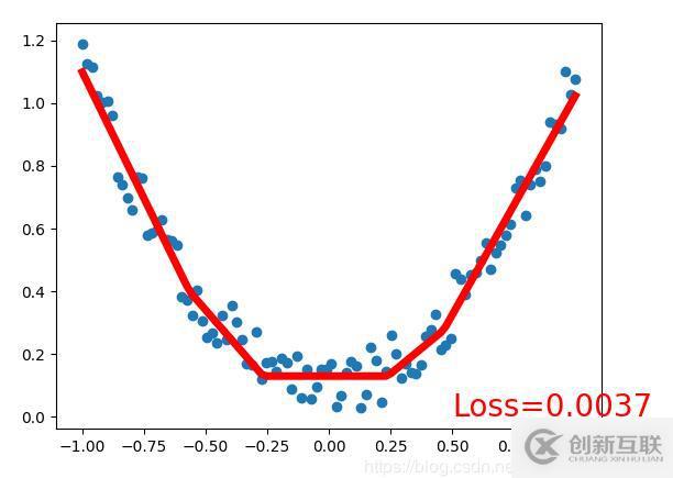

關(guān)于“Pytorch搭建分類回歸神經(jīng)網(wǎng)絡(luò)并使用GPU進(jìn)行加速的案例分析”這篇文章就分享到這里了，希望以上內(nèi)容可以對(duì)大家有一定的幫助，使各位可以學(xué)到更多知識(shí)，如果覺(jué)得文章不錯(cuò)，請(qǐng)把它分享出去讓更多的人看到。

新聞名稱：Pytorch搭建分類回歸神經(jīng)網(wǎng)絡(luò)并使用GPU進(jìn)行加速的案例分析-創(chuàng)新互聯(lián)
文章來(lái)源：http://chinadenli.net/article34/gecse.html

成都網(wǎng)站建設(shè)公司_創(chuàng)新互聯(lián)，為您提供網(wǎng)頁(yè)設(shè)計(jì)公司、網(wǎng)站內(nèi)鏈、網(wǎng)站制作、微信小程序、服務(wù)器托管、電子商務(wù)

廣告

聲明：本網(wǎng)站發(fā)布的內(nèi)容（圖片、視頻和文字）以用戶投稿、用戶轉(zhuǎn)載內(nèi)容為主，如果涉及侵權(quán)請(qǐng)盡快告知，我們將會(huì)在第一時(shí)間刪除。文章觀點(diǎn)不代表本網(wǎng)站立場(chǎng)，如需處理請(qǐng)聯(lián)系客服。電話：028-86922220；郵箱：631063699@qq.com。內(nèi)容未經(jīng)允許不得轉(zhuǎn)載，或轉(zhuǎn)載時(shí)需注明來(lái)源： 創(chuàng)新互聯(lián)